Factors Affecting the Vineyard Populational Diversity of Plasmopara viticola
Article information
Abstract
Vitis vinifera is very susceptible to downy mildew (Plasmopara viticola). A number of authors have suggested different genetic populations of this fungus exist in Europe, each showing a different degree of virulence. Work performed to date indicates this diversity to be the result of different factors. In areas where gene flow is greater and recombination more frequent, the diversity of P. viticola appears to be wider. In vineyards isolated by geographic barriers, a race may become dominant and produce clonal epidemics driven by asexual reproduction. The aim of the present work was to identify the conditions that influence the genetic diversity of P. viticola populations in the vineyards of northwestern Spain, where the climatic conditions for the growth of this fungus are very good. Vineyards situated in a closed, narrow valley of the interior, in more open valleys, and on the coast were sampled and the populations of P. viticola detected were differentiated at the molecular level through the examination of microsatellite markers. The populations of P. viticola represented in primary and secondary infections were investigated in the same way. The concentration of airborne sporangia in the vegetative cycle was also examined, as was the virulence of the different P. viticola populations detected. The epidemiological characteristics of the fungus differed depending on the degree of isolation of the vineyard, the airborne spore concentration, and on whether the attack was primary or secondary. Strong isolation was associated with the appearance of dominant fungal races and, therefore, reduced populational diversity.
For centuries, botrytis was the fungal disease that caused the greatest damage to the vineyards of the Old World. Abu Zacaria mentioned the disease in the 12th century (Abu, 1878), indeed, it was even known to Pliny the Elder (23–79 BCE). The end of the 19th century, however, saw the arrival from America of downy mildew (Plasmopara viticola), powdery mildew (Erisiphe necator), phylloxera (Dactylosphaera vitifoliae), and black-rot (Guignardia bidwelii), which together caused growers enormous losses. Given the length of time that botrytis (Botrytis cinerea) has been present in Europe, the genetic diversity shown by its populations is hardly surprising. However, after just over 100 years on the continent, wide genetic diversity is also being reported among P. viticola populations.
Today, downy mildew is the most serious of all grapevine diseases. It requires the greatest number of treatments, and thus has an economic impact beyond crop losses. The many applications of fungicide required also have negative environmental effects. Some authors report that in France, Italy, Greece, Australia and South Africa, genetically different populations - even different races - of this fungus exist that differ in their virulence (Delmotte et al., 2006; Délye and Corio-Costet, 1998; Evans et al., 1997; Koopman et al., 2007; Miazzi et al., 2003; Péros et al., 2005; Scherer and Gisi, 2006; Stummer et al., 2000). Delmotte et al. (2014) indicate that, over the last century, populations have appeared in Europe that differ from the original American invader.
Many authors (Chen et al., 2007; Delmas et al., 2016; Delmotte et al., 2014; Kast et al., 2001; Peressotti et al., 2010; Stark-Urnau et al., 2000) suggest that the diversity and different levels of virulence shown by P. viticola populations are the result of adaptation to growth on the varied grapevine varieties cultivated in Europe, to the reigning climatic and terrain conditions, and to the crop protection products used in different places. The opportunity for DNA recombination, and the ability to overcome plant resistance (as occurred with respect to cv. Bianca) (Delmas et al., 2016; Delmotte et al., 2011, 2014; Peressotti et al., 2010), may also play their part. Some authors (Fontaine et al., 2013; Gobbin et al., 2003a, 2003b, 2006, 2007; Koopman et al., 2007; Li et al., 2016) also suggest that P. viticola populations show greater genetic diversity during primary than during secondary infection.
The microsatellite markers (SSRs) developed by two research groups have long been used to study the genetic diversity of P. viticola. The first group of five SSRs, with 2–101 alleles per locus, was developed by Gobbin et al. (2003a). These markers were used to study different populations in Europe (Gobbin et al., 2003a, 2003b, 2005; Rumbou and Gessler, 2004, 2006), America (Kennelly et al., 2004, 2007), and Australia (Hug, 2005). Later, Delmotte et al. (2006, 2011) and Rouxel et al. (2012) between them developed 32 new SSRs with relatively low levels of polymorphism (1–6 alleles per locus). These markers have been used to characterise populations from Europe, North America, and more recently from China (Delmotte et al., 2006, 2011; Li et al., 2016; Rouxel et al., 2012; Yin et al., 2014, 2017; Zheng et al., 2017).
The Iberian Peninsula is home to some of the world’s greatest grapevine diversity. Many varieties are cultivated across areas with different edaphoclimatic and orographic conditions. However, no information is available on the diversity of disease-causing P. viticola for this territory. An analysis of this diversity in the Spanish northwest would be particularly interesting given the region’s environmental conditions, which are ideal for fungal development. The present work examines whether the genetic diversity shown by P. viticola in the vineyards of this part of Spain is influenced by isolation, the airborne spore concentration, and whether infection is primary or secondary.
Materials and Methods
Plant material and plot characteristics
This study was performed in four vineyard plots in northwestern Spain (Galicia) subject to different degrees of geographic isolation and different environmental conditions (Table 1, Fig. 1):

Plot locations, grape variety, altitude, years of plantation (YP), training systems, density of vines, distance between rows (dr), distance between grapevines in a row (dv), total nº plants (Np), plot surface area, sampling dates, and sample size (SS)
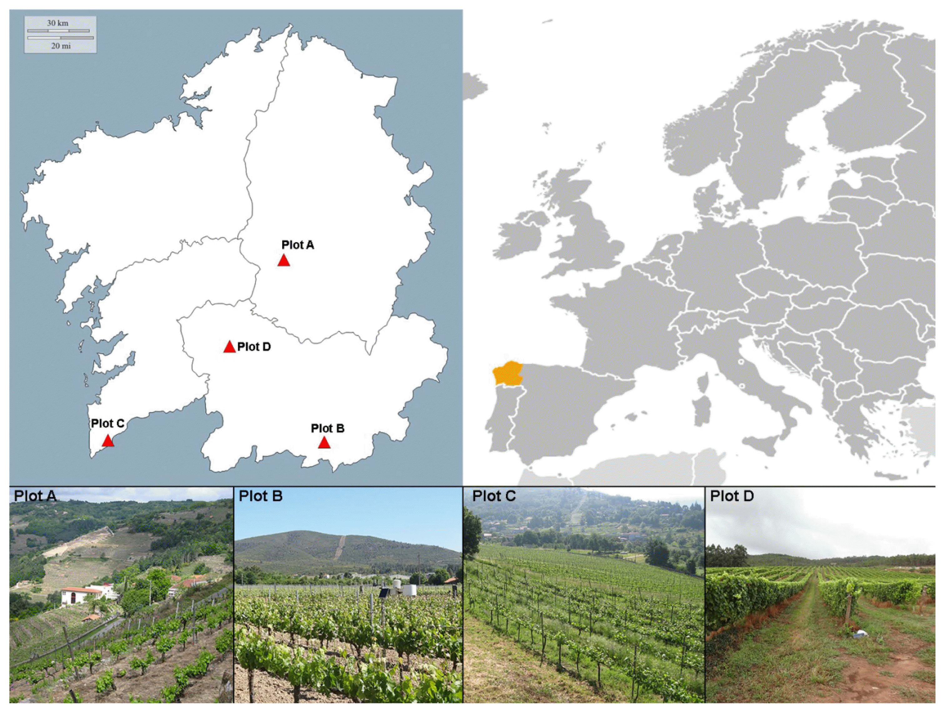
Plot locations and terrain type.
- Plot A: situated in a narrow, closed valley of the interior (strongly isolated); Denomination of Origin (D.O) area: Ribeira Sacra; variety grown = Mencia.
- Plots B and D: situated in more open valleys of the interior; D.O areas Monterrei and Ribeiro respectively; varieties grown = Dona Branca and Treixadura respectively
- Plot C: situated in open site on the coast; D.O area Rias Baixas subzone Rosal; variety grown = Albariño
In May and again in July of 2014, 30 leaves with symptoms of downy mildew (i.e., with primary infection symptoms in May [single sporulating lesions known as oil spots], and secondary infection symptoms in July [mosaic patches]) were collected from each plot (Table 1) for SSR analysis of the P. viticola present.
The experimental vineyard was tended to following standard production practices, except for the application of fungicides specific for, or with residual activity against, P. viticola. No treatments were applied to any plot, however, until all sampling for field susceptibilty to P. viticola (veraison) was finished.
Spore sampling
During the above sampling period, airborne spores (sporangia) of P. viticola were also collected in the different plots using sticky glass traps (four traps to a support stand) facing N, S, E and W (Fig. 2). Two supports were placed in each vineyard at different altitudes (if possible), and the traps (A and B) they carried at two heights (1 and 2 m) above the soil. All traps were replaced twice per month. Removed traps were examined by light microscopy (20× and 40×) after staining the sporangia with acidic lactofucsin (0.1% lactofucsin in lactic acid). Sporangia belonging to P. viticola were identified and the number in each trap noted.
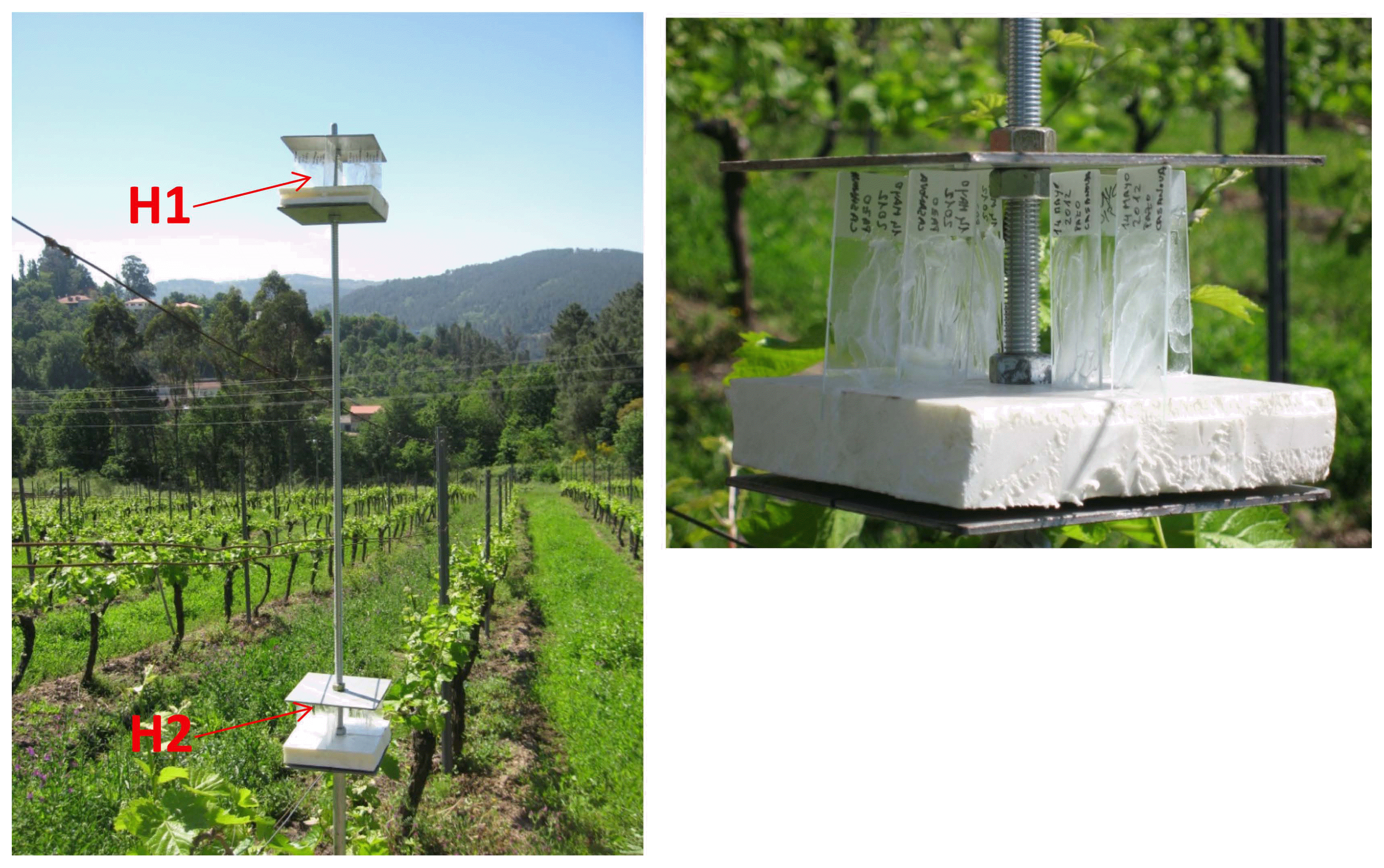
Airborne sporangia capture using sticky glass traps facing N, S, E and W. Two supports (A and B) were placed in each plot (at different altitudes if possible), and the traps they carried at two heights (H1 and H2 m) above the soil.
Susceptibility to downy mildew under field conditions
Between May and September 2014, the incidence of disease on the grapevine leaves and clusters in each plot was recorded using the method of Boso et al. (2005, 2011). Leaf and cluster symptoms were respectively examined 3 weeks after the onset of flowering and before veraison, in 20 plants per plot. In both cases, sampling was performed when more than 50% of the varieties showed symptoms of disease. Disease incidence was defined as the (number of leaves or clusters with symptoms/total number of leaves or clusters) × 100.
Weather monitoring
Soil temperature, air temperature (mean, maximum and minimum), leaf temperature, rainfall, relative humidity, solar radiation and other variables were measured using automatic μMCR200METOS agroweather stations (Pessl Instruments Ltd., Weiz, Austria) in each plot over the study year (2014).
DNA extraction and marker selection
Frozen tissue of each sample was disrupted using a Retsch ®Mixer Mill MM 300 (Retsch GmbH, Haan, Germany) and DNA isolated using the Qiagen DNeasy Plant Mini Kit (Qiagen, Basel, Switzerland). It was then quantified in a Nanodrop 2000 spectrophotometer (Thermo Scientific, Wilmington, DE, USA), and its integrity confirmed in agarose gels.
The presence of P. viticola DNA was examined by amplifying the GIOP marker (Valsesia et al., 2005). Genetic variation among the fungal samples was analyzed by PCR amplification of the ISA, CES, GOB, BER, Pv13, Pv17, Pv31 microsatellites (Delmotte et al., 2006; Gobbin et al., 2003b).
PCR amplification and genotyping
Amplification was performed in a Bio-Rad MyCycler Thermal Cycler (Bio-Rad Laboratories, Hercules, CA, USA), using 1 μl of extracted DNA, 1 U of Kapa Taq (Kapa Biosystems, Boston, MA, USA), 0.32 mM of total dNTP, 0.08 μmol of each labelled forward primer (BER-F and ISA-F labelled with D2 dye, Pv13-F, Pv17-F and Pv31-F with D3 dye, and GOB-F and CES-F with D4 dye [Invitrogen, Inchinnan, Scotland, UK]), 0.25 μmol of non-labelled forward primers, and 0.4 μmol of the reverse primers (see Supplementary Table 1 for full information on primers), adding PCR buffer (10 mM Tris-HCl pH 7.2, 50 mM KCl) to a final reaction volume of 20 μL. The reaction conditions were as follows: an initial cycle of 95°C for 5 min, followed by 38 cycles of 30 s at 95°C, 30 s at 56–58°C (depending on the primer pair; see Supplementary able 1), 50 s at 72°C, and a final extension of 10 min at 72°C.
The resulting amplicons were separated in a 6% acrylamide/bis-acrylamide (19:1) gel in the presence of Gel Red® Gel-Red (Biotium, Hayward, CA, USA) to confirm the presence of amplicons in each sample. Gel images were digitalized using the VisiDoc-it™ Imaging System 6.4 LCD system and visualized using Quantity One v.4.6.6 software (BioRad Laboratories, Hercules, CA, USA). 0.5 μl of the amplified fragments (1 μl for the GOB fragment) were run in an automatic sequencer with 40 μl of deionised formamide (Beckman-Coulter, Krefeld, Germany) plus a D1-labelled 60–420 bp CEQ DNA size standard (Beckman-Coulter, Krefeld, Germany) to determine the fragment sizes. These sizes were assigned using a CEQ 8800 Genetic Analysis System (Beckman-Coulter).
Statistical analysis
The heterozygosity, polymorphism information content (PIC), number of expected and observed alleles, and the diversity for each microsatellite locus, was examined using PowerMarker v.3.25 software (Liu and Muse, 2005). GeneAlex v.6.5 software (Peakall and Smouse, 2006, 2012) was used to calculate the Nei genetic distances among populations, along with other population genetics indices. Microsoft® Excel 2007/XLSTAT© v.2016.04.32217 software (Addinsoft, Inc., Brooklyn, NY, USA) was used to conduct principal coordinates analysis (PCA) in order to examine the genetic relationships among and within populations.
Results and Discusion
Table 2 shows the maximum and minimum temperatures, the mean temperature, rainfall and relative humidity (RH) values for the different plots. Plot C showed the most favourable climatic conditions for fungal growth over the sampling period (RH 70–75%, rainfall 62.2–105.2 mm Tmax < 27°C) (Gessler et al., 2011). The conditions in Plot B were less favourable (RH 60–65%, rainfall 26.2–37.6 mm, Tmax 30–37°C).
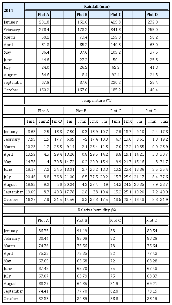
Monthly temperature (°C), rainfall (L/m2) and relative humidity (%) at the plots
Airborne sporangia
In general, the highest airborne sporangia concentrations were recorded in May in all plots. Plot D had the highest concentration, followed by B, C, and A (Table 3, Fig. 3).

Airborne sporangia concentrations (mean and standard deviation)
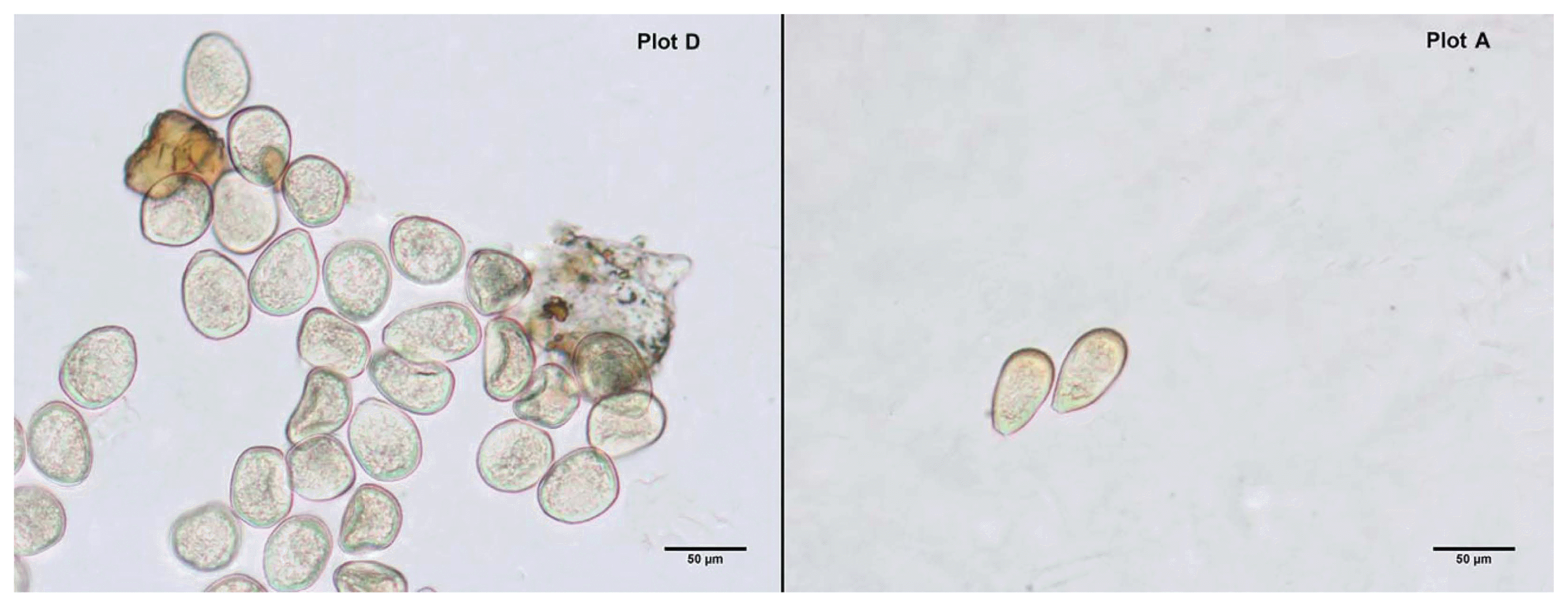
Micrographs of airborne sporangia (magnification 40×). Plot D had the highest concentration, and Plot A the lowest.
Susceptibility to downy mildew under field conditions
The damage caused by downy mildew in the study period was less than that normally seen in the plot areas. The high and low temperatures at different moments in the growth cycle limited the development of P. viticola (especially in June and July in Plots A, B and D). In these plots, symptoms of disease were seen on both the leaves and clusters, although disease incidence was < 25%. In Plot C, disease incidence was > 25%, and reached 70% in early sampling (primary infection) (Table 4). It may be that the fungal population affecting Plot C was more aggressive than those in the other plots, or that the grapevine variety in Plot C (Albariño) was more susceptible. Kast (2001) suggests that fungal ‘races’ show different levels of aggressiveness depending on the grapevine host variety, i.e., different genetic populations of P. viticola show greater affinity towards some varieties than others. Our group is currently studying this possibility.

Mean disease incidence (%) under field conditions observed on leaves and clusters
Identification of P. viticola and genotyping
Amplification of the GIOP marker confirmed P. viticola to be present in amplifiable quantities in 68 of the 240 leaf samples collected. Table 5 shows that Plots C and D (those with the highest incidence of disease) returned the highest proportions of infected leaves (both primary and secondary infections). Plots C and D (especially) also returned the largest number of airborne sporangia.

Allele diversity and possible fungal genotypes
SSR analysis returned a different number of alleles for each plot, depending on the marker in question. Table 6 shows the number of alleles, number of genotypes, major allele frequency, heterozygosity, and PIC etc. for each SSR and plot (primary+secondary infection). GOB was expected to be the most polymorphic marker, as indicated by the size range of the amplicons (Supplementary Table 1). Forty nine GOB alleles and 116 different GOB genotypes were identified (Table 6). The PIC value for this marker was 0.94. The GOB allele number for the different plots and for primary and secondary infection ranged from 3 to 20 - sometimes with as many as 7 alleles recorded for the same sample (Table 5). When combinations of alleles were generated to determine the number of different fungal populations present in each sample, the GOB marker returned up to 54 - which hardly seems realistic. It would seem that despite being a very informative SSR marker (Gobbin et al., 2003b), GOB is not so valuable in analyses of population genetics, at least in the present setting. GOB was therefore left out of all subsequent analyses. The total possible number of fungal genotypes was therefore generated using the remaining markers. CES returned the highest number of alleles (14), and the highest PIC (0.77), but the lowest allele frequency for the major allele (0.33) (Table 6). Pv13 and Pv31 were not very polymorphic, returning PICs of 0.19 and 0.31 respectively.

Number of alleles and genotypes, observed heterozygosity, gene diversity and polymorphism information content (PIC) of the seven P. viticola SSR loci
All plots showed similarities with respect to the percentage of polymorphic loci, the number of effective alleles, and the unbiased expected heterozygosity for all the SSRs (GOB) taken together (Table 7). The number of genotypes detected for the primary and secondary infection populations differed greatly between plots: Plot A had 7 primary and 3 secondary infection genotypes, Plot B had 5 primary and 5 secondary infection genotypes, Plot D had 23 primary and 37 secondary infection genotypes, and Plot C had 18 primary and 28 secondary genotypes. These differences may have several explanations, but in Plot D the most important influence may have been the high airborne spore concentration (Table 3). In addition, Plots D and C were those with the greatest incidence of disease, which may have provoked the appearance of more genotype diversity.

Summary of population genetics indices
Plot A was located on a steep, terraced slope (> 30%) of a closed, narrow valley. It might be speculated that, in such an environment, air currents that would bring in fungal spores may have been restricted, effectively isolating the vineyard from inward gene flow and reducing the diversity. This might facilitate the appearance of dominant fungal races that produce clonal epidemics driven by asexual reproduction (Koopman et al., 2007; Rumbou and Gessler, 2004, 2006). The other three vineyards were flatter, although each had its peculiarities. Plot B was far away from other vineyards and surrounded by houses; it too was therefore isolated. The remaining plots, C and D, were open and surrounded by other vineyards; it was in these plots that the greatest populational diversity was seen, perhaps due to the free movement of spore-carrying air currents. This would have promoted gene flow between the populations, giving rise to more opportunities for genetic recombination. It should be remembered that the climatic conditions of Plot C were more propitious for the growth of P. viticola. In plots A, B and D the temperature surpassed 30°C in June and July (the time of secondary infections), inhibiting fungal growth. This could have reduced the appearance of diversity.
The plot with most genotypes also had the highest number of private alleles, except for the primary infection samples from Plot B, which had five fungal haplotypes and just one private allele (Table 7). The Shannon index was in general low and very similar for the different plots; the highest values were obtained for secondary infection samples from Plots B and D. It is remarkable that the samples from Plots D and C showed mainly negative fixation index values, while Plots A and B returned positive values. These results agree with the proportions of observed heterozygotes, which was greater than expected for the former two plots and smaller than expected for the latter two. The genetic differentiation reflected by the fixation index also reveals that the genetic structure might be related to the degree of plot isolation due to the surrounding geographical barriers. The genotypes in Plot A largely correspond to dominant races that produce clonal epidemics driven by asexual reproduction.
To examine the development of the infection over time, PCA was performed for each plot separately, taking into account primary and secondary infection individually. These analyses showed the first three axes to explain from 70.55% (Plot D) to 89.96% (Plot A) of the variance. The fungal populations of Plot C grouped by primary and secondary infection, but this was not seen for the other plots (Fig. 4). The populations associated with secondary infection in Plot C might not have arisen from those involved in primary infections, but from spores arriving on air currents from elsewhere. They may also have appeared as the result of recombination, or, as some authors suggest (Jermini et al., 2003, 2009; Matasci et al., 2008), have been the product of oospores that had remained latent in the soil until June.
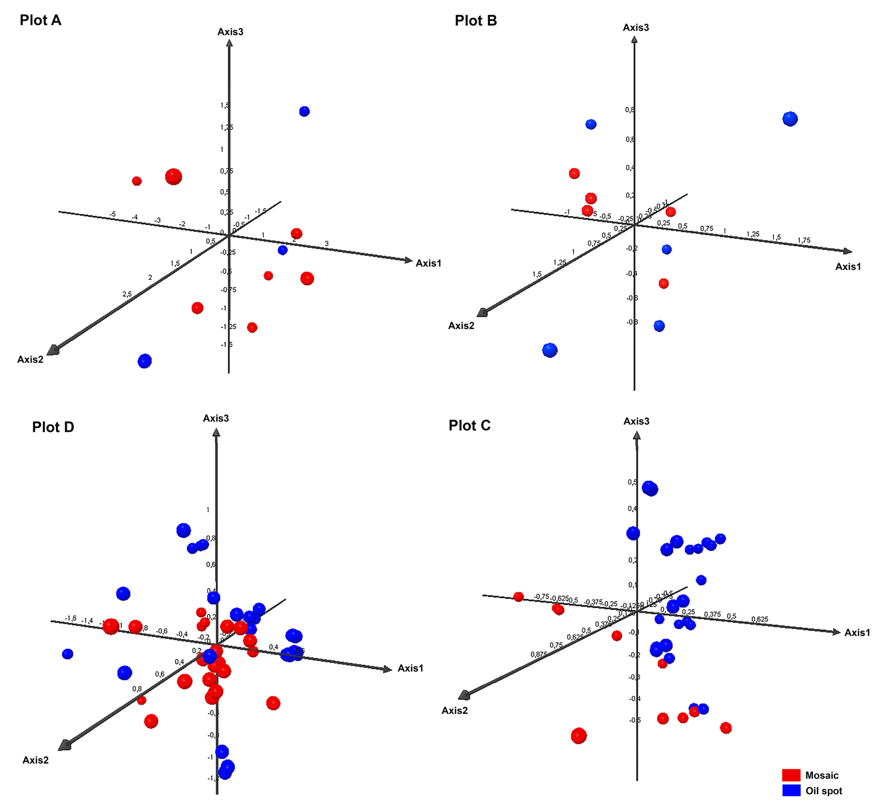
PCA performed for each plot separately, taking into account primary (oil spot) and secondary infection (mosaic spot).
Some authors (Jermini et al., 2009; Pertot and Zulini, 2003) report the existence of greater genetic diversity for P. viticola during primary infection. In the present work, however, this was only observed for the most isolated plot, Plot A. In fact, in Plots C and D, more genetic diversity was seen during the period of secondary infection.
Table 8 shows the pairwise population matrix for the Nei genetic distances between the plots. The largest genetic distances were between Plot C and Plots A/B, both for primary and secondary infection. The smallest genetic distance was between Plots A and B, both for both primary and secondary infection; in fact, the intraplot distances for both primary and secondary infection were larger.
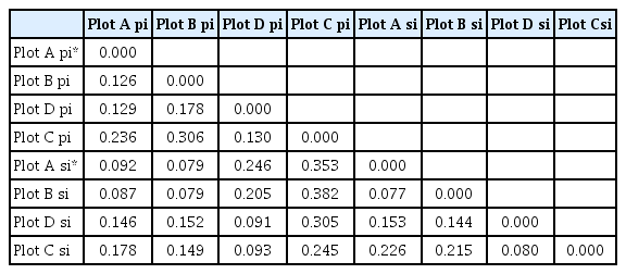
Pairwise population matrix for Nei genetic distances (pi = primary infection; si = secondary infection)
In conclusion, wide populational diversity was detected for P. viticola. The epidemiological characteristics of each plot were driven by factors such as the degree of isolation, the airborne spore concentration, and by whether the infection was primary or secondary. This agrees with observations of other authors that different races of P. viticola exist in different vineyards across Europe (Gobbin et al., 2003b, 2006; Stark-Urnau et al., 2000). The appearance of dominant races would appear to be a consequence of isolation (Koopman et al., 2007; Rumbou and Gessler, 2004, 2006).
Supplementary Information
Acknowledgments
This work was funded by the Fundación Juana de Vega. The authors thank the Adegas Moure (D.O. Ribeira Sacra), Bodega Terras Gauda (D.O. Rias Baixas, subzone O Rosal), Félix Estévez (D.O. Monterrei) and Bodegas Pazo Casanova (D.O. Ribeiro) wineries for their collaboration, and Iván González and Elena Zubiaurre for technical assistance.